Analyzing Llama-3 weights via RMT
Prerequisite: Marchenko-Pastur (MP) Law
Definition
For \(A \in \mathbb{R}^{m,n}\) with IID entries sampled with \(\sigma \in \mathbb{R}^+\), the PDF of the singular values of \(\frac{1}{m}AA^T\) is given by:
\[\begin{aligned} P_{\mathrm{MP}}(\nu) & = \begin{cases}\frac{n / m}{\pi \tilde{\sigma}^2 \nu} \sqrt{\left(\nu_{\max }^2-\nu^2\right)\left(\nu^2-\nu_{\min }^2\right)} & \nu \in\left[\nu_{\min }, \nu_{\max }\right] \\ 0 & \text { else }\end{cases} \\ \nu_{\min } & =\tilde{\sigma}(1 \pm \sqrt{m / n}), \quad \tilde{\sigma}=\sigma \sqrt{n} . \end{aligned}\]This PDF depends exclusively on the dimension of the matrix \((m,n)\) and the \(\sigma\) that they’re sampled from.
Plots for Kaiming initialized matrices
Kaiming initialization is a common initialization scheme used in neural networks. Functionally, it works by sampling each value of your weight matrix from \(\mathcal{U}(-bound, bound)\), where \(bound\) is calculated as:
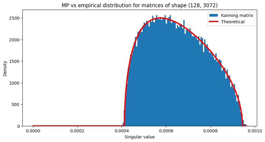
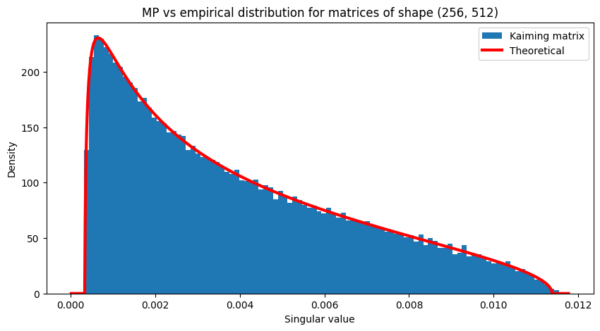
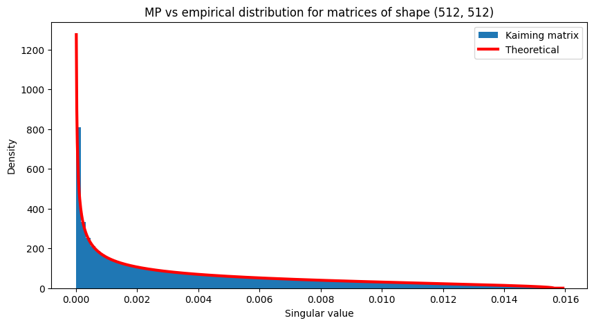
\[bound = gain \times \sqrt{\frac{3}{\text{fan_mode}}}\]In the below plots, I’ve plotted the MP distribution for a few matrix shapes (in red) versus the empirical distribution of singular values when the matrices are initialized with kaiming initialization:
Using deviation to MP as a qualitiative proxy for how close a matrix is to initialization
By comparing the histogram of a matrix’s singular values to the MP distribution, we can qualitatively measure how far a matrix is from initialization by seeing how far the histogram is from the red curve. They match as we would expect.
Summary of “Locating Information in Large Language Models via Random Matrix Theory “ by Staats et al.
This paper introduces the idea of analyzing BERT and Llama by qualitatively seeing differences in the MP distribution on averaged Llama 3 and BERT matrices.

As you can see above, we see that output projection matrices are closer to the MP distribution compared to queries on average.
They also introduce a way of measuring the randomness of a matrix using a Kolmogorov-Smirnov test (explained later).

The x-axis is the index of the singular vector for the given layer. The Y axis is the P-value. The higher the P-Value, the closer the singular vector is to being “random”. In thier paper, they use this to find “outlier” singular vectors, but in my case I’ve repurposed it as a measure of randomness of an entire matrix.
Analyzing Llama-3.2 with RMT
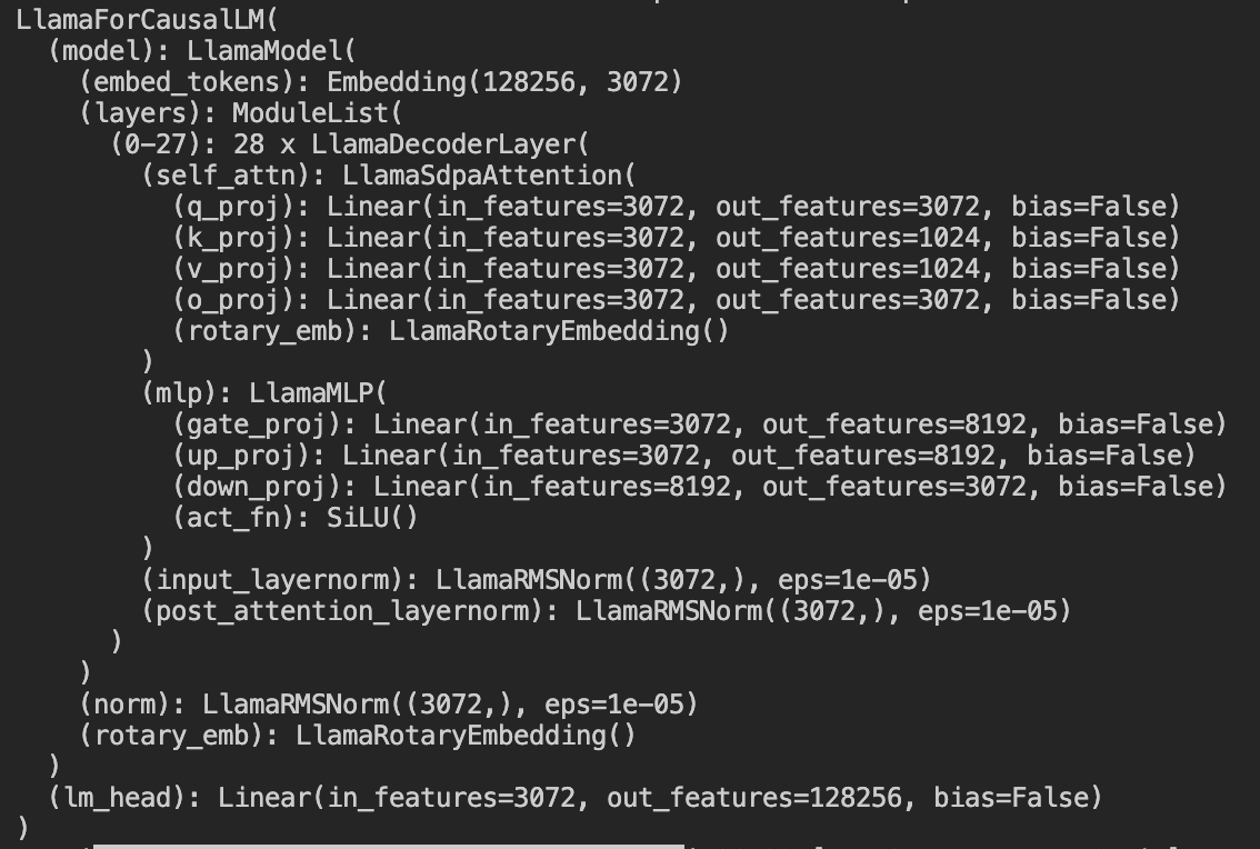
In this work, we’ll anaylze the multi-head query, key and value matrices (q_proj, k_proj, v_proj).
Analyzing the query matrix across heads and layers
If we plot the query matrix for an early layer in the network, we get the following plot:
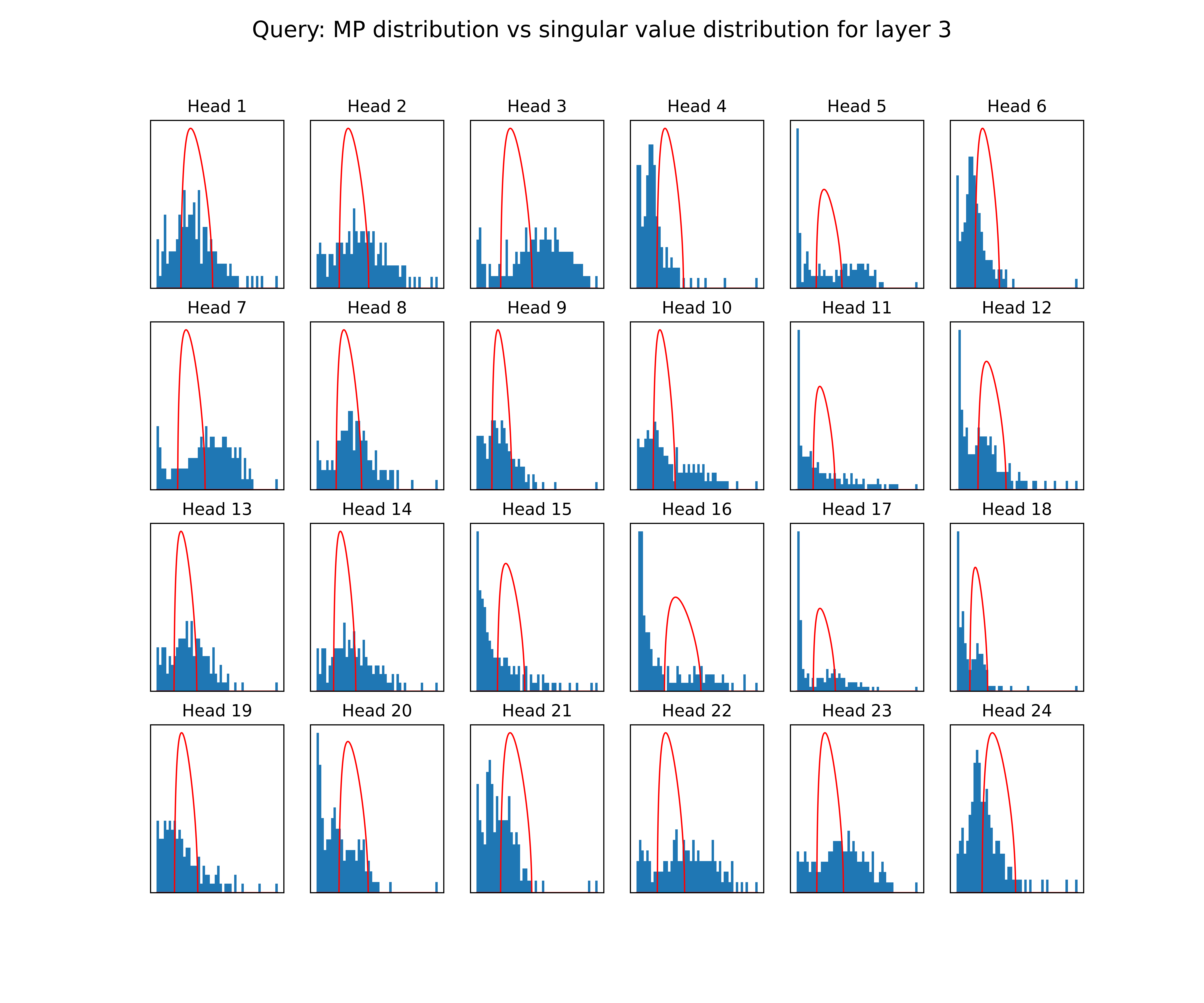
Recall the red curve is the MP distribution and the histogram is the distribution of singular values, so this means that the heads in this layer are very far from initialization (the MP distribution).
Let’s repeat this for a later layer:
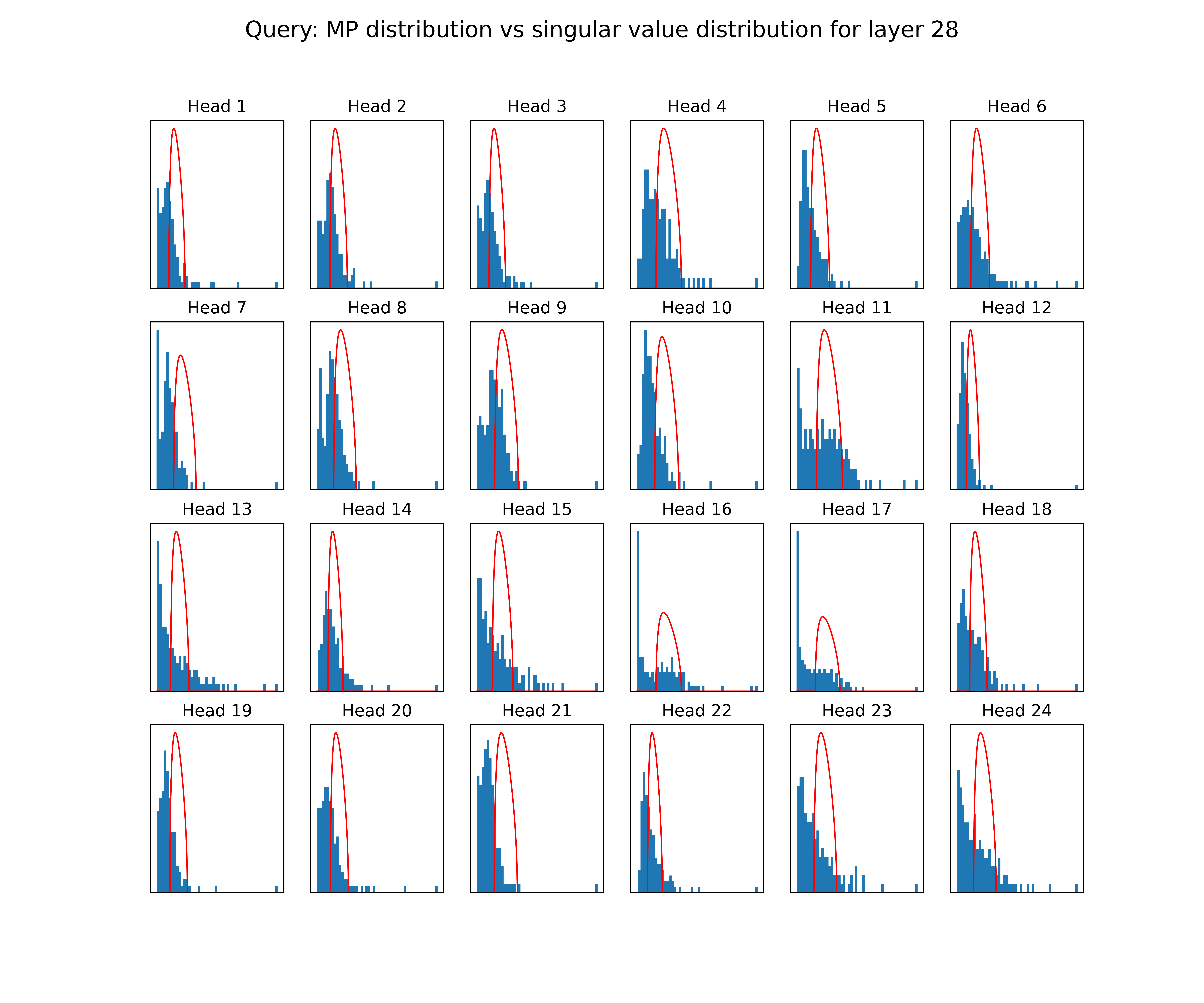
As you can see, we have that the later layers are a lot closer to the theoretical MP distribution compared to the early ones.
Quantitative assessment of randomness via Kolmogorov–Smirnov test
Given that the matrix has IID entries and finite variance, the entries of its singular vectors \(v\) of size \(n\) should follow a standard normal distribution with an std of \(\frac{1}{\sqrt{n}}\)
\[P\left(v_i\right)=\frac{1}{\sqrt{2 \pi / n}} \exp \left(-\frac{1}{2} v_i^2 n\right)\]This lets us perform a Kolmogorov-Smirnov test via a theoretical gaussian CDF:
\[C_{\mathrm{G}}(x)=\frac{1}{2}+\frac{1}{2} \operatorname{erf}(\sqrt{n / 2} x)\]In our case, I compute the P-Value for EACH singular vector in each head, and then I average those to get a single statistic for each head. I then average again to get a single statistic for each layer. Once this is done, we get the following plots:
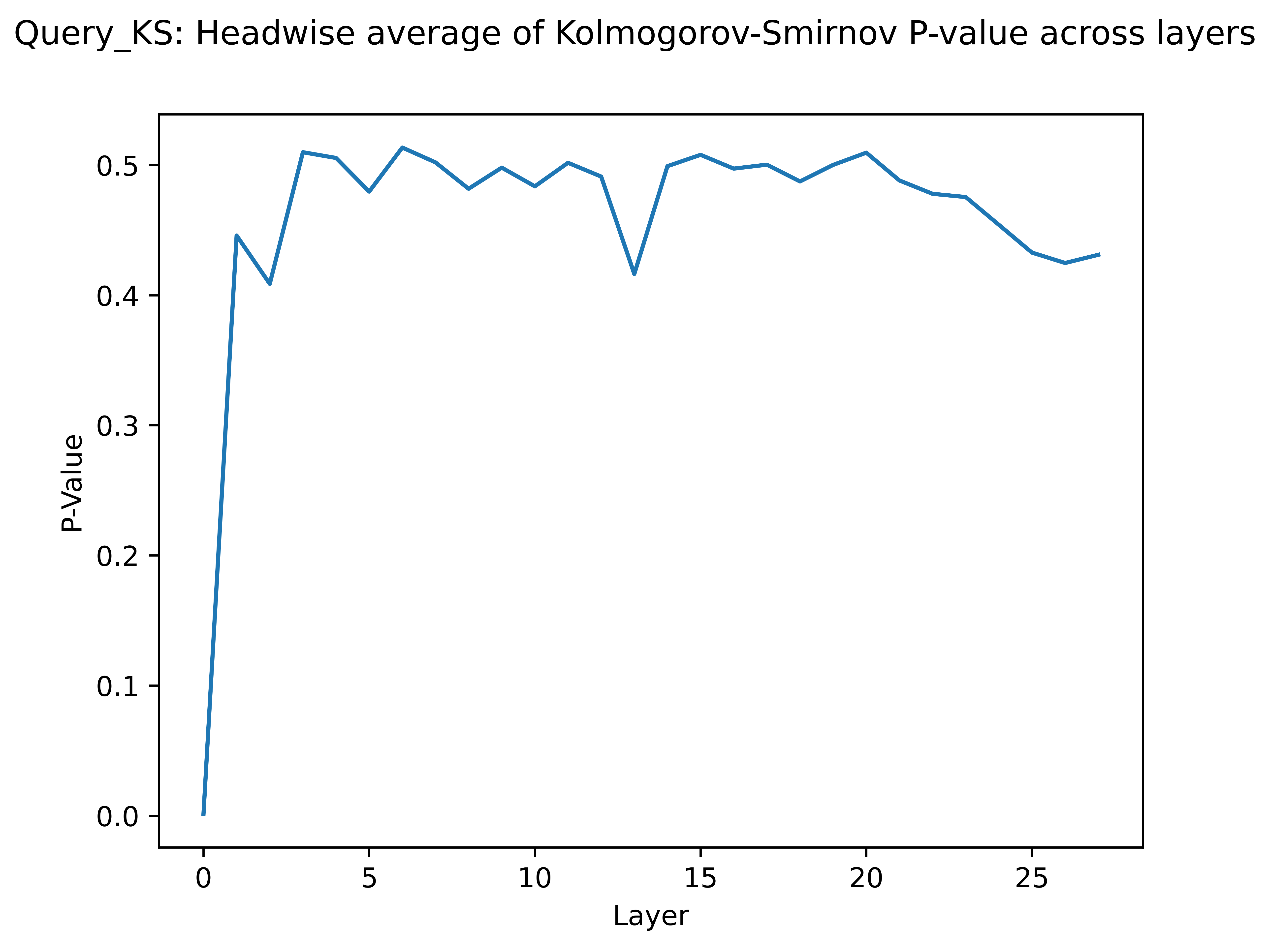
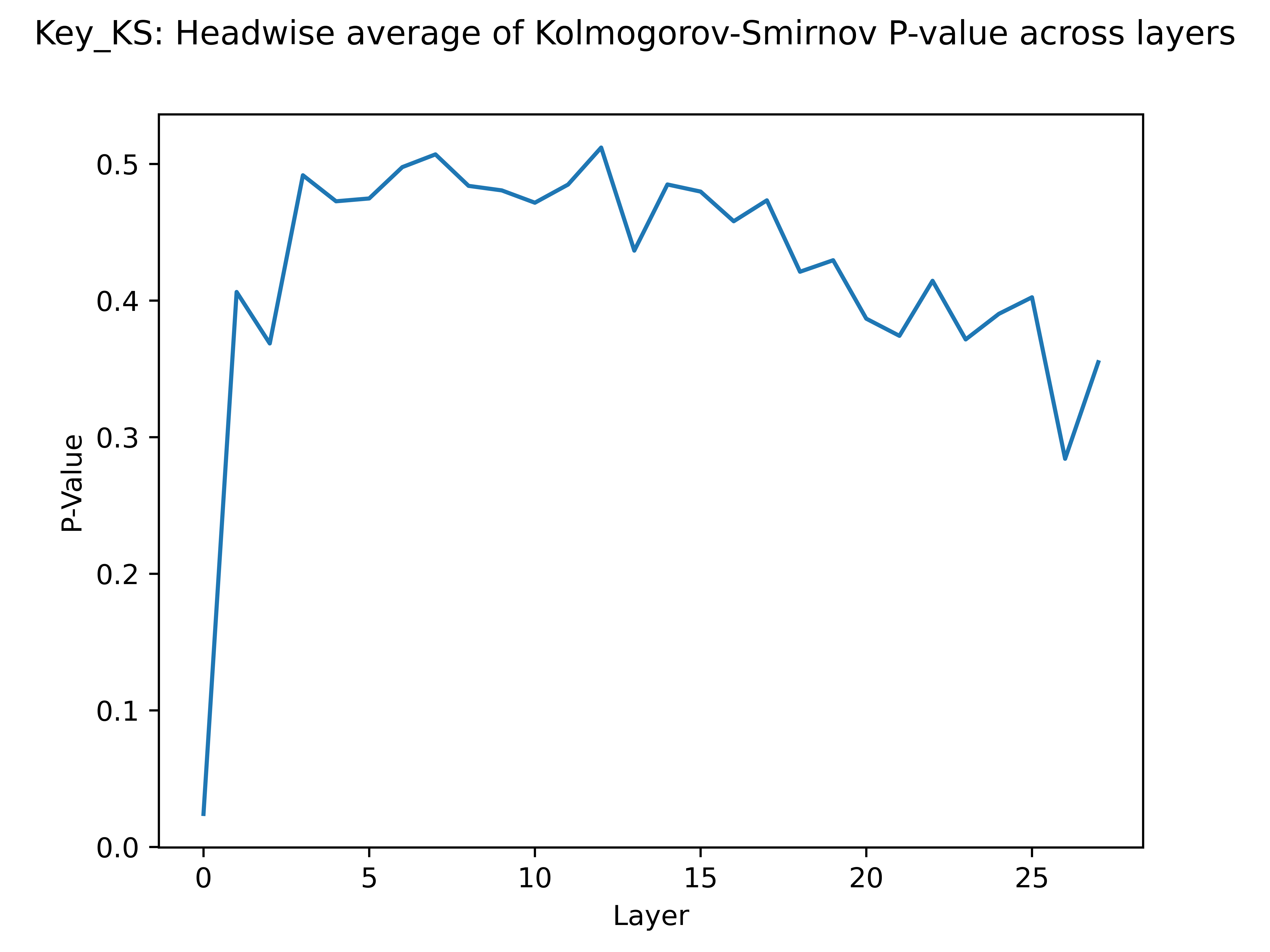
As you can see, the “randomness” of the weight matrices shoots up as a function of depth. Though I expected to see a linear relationship between layer and p-value, we can see instead that it saturates quite fast as we go deeper into the network.
Conclusion
All I’ve really found evidence for is that the first few (1-5) layers of Llama 3.2 are very far from random init, and the later and middle layers of the network tend to be closer to random init.
This method of showing such a phenomenon may be slighly exotic, but the results mentioned above aren’t new at all and have been found time and time again in the deep learning community.
One example of this are papers that show you can chop off penultimate layers of a neural network and achieve minimal performance hits.