Deriving the ELBO for VAEs
Assume we have some log likelihood \(\log(p_\theta(x))\) we want to maximize, where the parameters of our probablistic model can be denoted as \(\theta\). Now, we express it in terms of joint probability of \(p_\theta(x, z)\) as:
\[\log \left ( \int_z p_\theta (x,z) dz \right )\]We call \(z\) a “latent variable”. In the case that we have multiple latent variables in a vector \(\mathbf{z} \in \mathbb{R}^n\), we can write
\[\log \left ( \int_\mathbf{z} p_\theta (x,z_1, z_2, \dots, z_n) d\mathbf{z} \right )\]This is intractable, as this requires way too many \(\mathbf{z}\) values to get a good enough approximation.
Hence, if we lower bound this with something that IS tractable, then we’re able to optimize this.
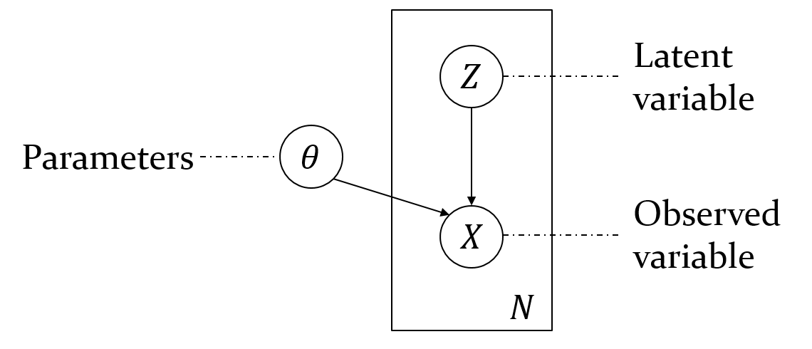
Since we have a joint probability \(p_\theta(x, \mathbf{z})\), we want to somehow decompose this into a product of two probabilities using the product rule. Below, you can see the graphical model, which tells us how we should be decomposing the joint distribution.

Therefore by decomposing the joint according to the graphical model:
\[= \log \left( \int_{\mathbf{z}} p_\theta (x \mid \mathbf{z}) p(\mathbf{z}) d\mathbf{z} \right )\]We refer to \(p(\mathbf{z})\) as the “prior”, which is a distribution over our latent variables. Notice I don’t subscript this with \(\theta\), because it doesn’t have any paramters and is just a fixed distribution.
Now, I will make a distinction. There are two distributions we are trying to learn: \(p(x \mid \mathbf{z})\) and \(p( \mathbf{z} \mid x)\). Overriding my previous notation, I denote \(\theta\) as the parameters for \(p_\theta(x \mid \mathbf{z})\) and \(\phi\) as the parameters for \(p_\phi(\mathbf{z} \mid x)\).
Hence, going back to the log-likelihood, I multiply the insides by \(\frac{p_\phi (\mathbf{z} \mid x)}{p_\phi (\mathbf{z} \mid x)} = 1\).
\[= \log \left( \int_{\mathbf{z}} p_\theta (x \mid \mathbf{z}) p(\mathbf{z}) \cdot \frac{p_\phi (\mathbf{z} \mid x)}{p_\phi (\mathbf{z} \mid x)} d\mathbf{z} \right )\]Then, I convert this into an expectation:
\[\log \left( \mathbb{E}_{\mathbf{z} \sim p_\phi (\mathbf{z} \mid x)}\left [ p_\theta (x \mid \mathbf{z}) \cdot \frac{p(\mathbf{z})}{p_\phi (\mathbf{z} \mid x)} \right ]\right )\]At this point, we can apply jensen’s inequality, which tells us that \(\log \left( \mathbb{E}\left [X \right] \right ) \geq \mathbb{E}\left [\log(X) \right]\). Applying this gets us:
\[\log \left( \mathbb{E}_{\mathbf{z} \sim p_\phi (\mathbf{z} \mid x)}\left [ p_\theta (x \mid \mathbf{z}) \cdot \frac{p(\mathbf{z})}{p_\phi (\mathbf{z} \mid x)} \right ]\right ) \geq \mathbb{E}_{\mathbf{z} \sim p_\phi (\mathbf{z} \mid x)}\left [ \log \left( p_\theta (x \mid \mathbf{z}) \cdot \frac{p(\mathbf{z})}{p_\phi (\mathbf{z} \mid x)} \right ) \right ]\]I will then simplify the right side:
\[\begin{align*} &= \mathbb{E}_{\mathbf{z} \sim p_\phi (\mathbf{z} \mid x)} \left [ \log \left( p_\theta (x \mid \mathbf{z}) \right) + \log \left( p(\mathbf{z}) \right) - \log \left (p_\phi (\mathbf{z} \mid x) \right ) \right ] \\ &=\mathbb{E}_{\mathbf{z} \sim p_\phi (\mathbf{z} \mid x)} \left [ \log \left( p_\theta (x \mid \mathbf{z}) \right) \right ] + \mathbb{E}_{\mathbf{z} \sim p_\phi (\mathbf{z} \mid x)} \left [ \log \left( p(\mathbf{z}) \right) \right ] - \mathbb{E}_{\mathbf{z} \sim p_\phi (\mathbf{z} \mid x)} \left [ \log \left (p_\phi (\mathbf{z} \mid x) \right ) \right ] \\ &=\mathbb{E}_{\mathbf{z} \sim p_\phi (\mathbf{z} \mid x)} \left [ \log \left( p_\theta (x \mid \mathbf{z}) \right) \right ] - \text{KL} \left[ p(\mathbf{z})\mid \mid p_\phi (\mathbf{z} \mid x) \right ] \end{align*}\]Where \(\text{KL}\) is the \(\text{KL}\) divergence between the prior \(p(\mathbf{z})\) and the posterior \(p_\phi(\mathbf{z} \mid x)\)