Turning your diffusion model into a classifier
In this post, we’ll be going over the “Your Diffusion model is secretly a zero-shot classifier” paper (https://arxiv.org/abs/2303.16203).
Diffusion model recap
The main idea of a diffusion model is that we’re learning an approximation to the true data distribution called \(p_\theta(x_0)\) by maximimizing an ELBO:
\[p_\theta(x_0) \geq - \mathbb{E}_{t, \epsilon} \left [ || \epsilon - \epsilon_\theta (x_t)||^2 \right ]\]If we want to do conditional diffusion, we simply can add a condition vector \(c\), and model the conditional
\[p_\theta(x_0 \mid c) \geq - \mathbb{E}_{t, \epsilon} \left [ || \epsilon - \epsilon_\theta (x_t, c)||^2 \right ]\]Bayesian flippy flip
Say we’ve learned \(p_\theta(x \mid c)\), how do we turn this into a classifier? Well, we’ll need to model \(p_\theta(c \mid x_0)\).
Here is the key derivation:
\[p_\theta(c = c_i | x_0) = \frac{p(c_i)p_\theta(x_0 \mid c = c_i)}{\sum_j p(c = c_j)p_\theta(x_0 \mid c = c_j) }\]However, since we were kids, we’ve been told that \(p_\theta(x_0 \mid c)\) is NOT tractable! Thankfully, ELBO (when tight enough) is basically equal to \(\log p_\theta (x_0 \mid c)\).
Therefore, we can simply sub our ELBO into this and get:
\[p_\theta\left(c = c_i \mid x_0 \right)=\frac{\exp \left\{-\mathbb{E}_{t, \epsilon}\left[\left\|\epsilon-\epsilon_\theta\left(x_t, c_i\right)\right\|^2\right]\right\}}{\sum_j \exp \left\{-\mathbb{E}_{t, \epsilon}\left[\left\|\epsilon-\epsilon_\theta\left(x_t, c_j\right)\right\|^2\right]\right\}}\]You can approximate the expectation by using monte carlo sampling given a datapoint \(x\) and conditioning inputs \(\{c_i \}_{i=1}^n\) using the following steps:
Firstly, create a list \(\text{Error}[c_i] = 0\), for each \(c_i\).
Then, for \(N\) trials,
-
Sample \(t \sim \text{Unif}[1, T]\), and \(\epsilon \sim \mathcal{N}(0,I)\).
-
Forward diffuse \(x_t = \sqrt{\bar{\alpha_t}}x + \sqrt{1 - \bar{\alpha_t}} \epsilon\)
-
For each conditioning input \(c_k \in \{c_i \}_{i=1}^n\), accumulate the loss as \(\text{Errors}[c_k] := \text{Error}[c_k] + \| \epsilon - \epsilon_\theta (x_t, c_k) \|^2\).
Finally, after all this is over, you can simply compute class assignments by:
\[c = \text{argmin}_{c_i}(\text{Error}[c_i])\]Or you can just throw it all into a softmax to get a categorical distribution:
\[p_\theta(c | x) = \text{Softmax}(\text{Error})\]Toy experiment
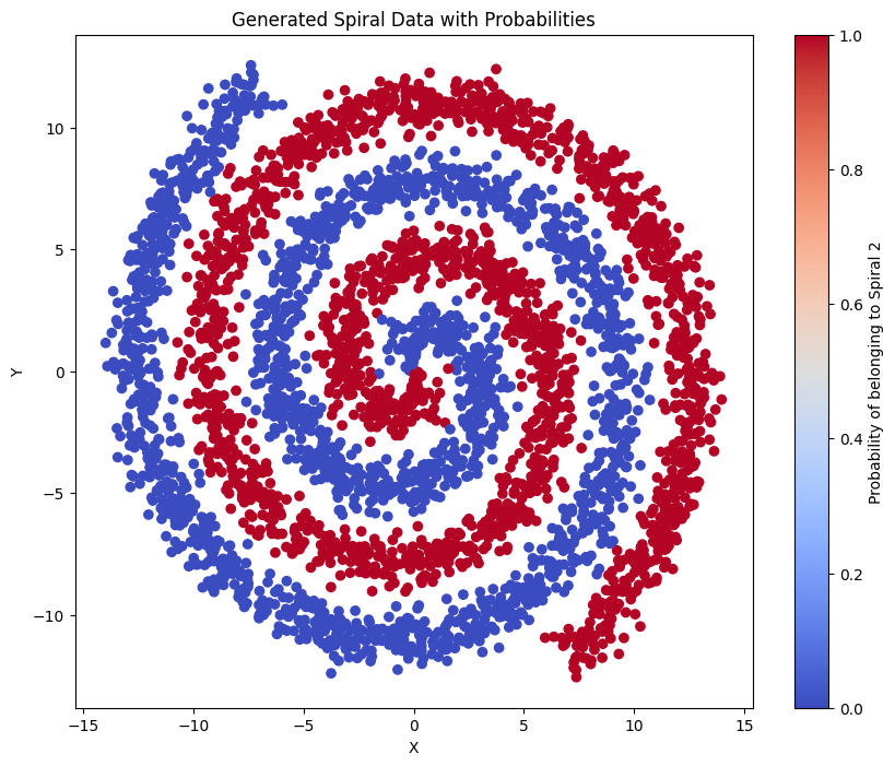
Let’s start with some data of two interlaced spirals (classes are red and blue):

Next, let’s train a diffusion model on this conditional data. Below is an example generation after it’s trained, where the red points are random noise conditioned on the red class and blue points are random noise conditioned on the blue class.
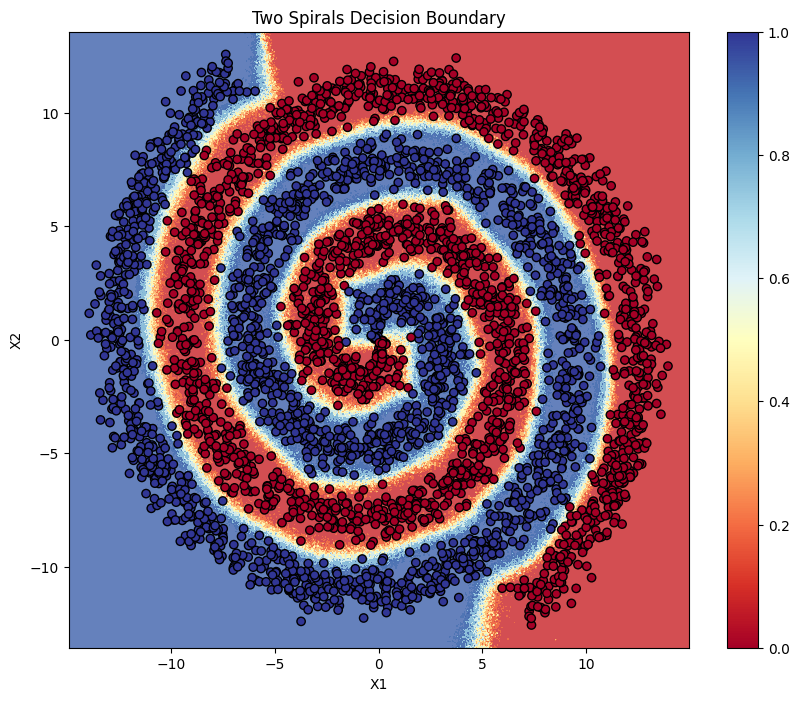
Here’s the decision boundary of our classifier:

It works pretty decently!