Road to modern SSL Part 1, Ensembles, crops and augmentations
I want to study each of a modern SSL pipeline’s components in isolation, until I’m able to understand the origins/reasoning for throwing all the components together.
In this post, we’ll be studying the rationale and development of using an exponential moving average (EMA) of a neural network during SSL training.
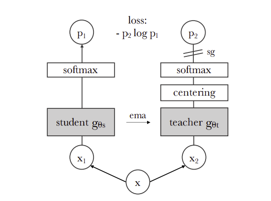
EMA is often used as a “teacher network”, for example see this figure from the DINO paper below:
Origins in deep learning
The first time I saw EMA was when I was reading the ADAM optimizer paper, where they kept an EMA of the gradients.
EMA is defined as the following for some parameter \(\beta\in (0, 1)\):
\[v_t = \beta v_{t-1} + (1-\beta) o_t\]Where \(v_t\) is our state at time \(t\) and \(o_t\) is our observation at timestep \(t\).
Normally, we init with \(v_0 = 0\), this means our first “state” is going to be \(v_1 = (1-\beta)o_1\). With most choices of beta, this will be a downscaled version of the first observation.
Therefore, we apply some bias correction by dividing our update rule by \((1-\beta^t)\):
\[v_t = \frac{\beta v_{t-1} + (1-\beta) o_t}{1-\beta^t}\]The denominator quickly goes to ~1 and has no effect for future values of \(t\). But atleast for the first iteration, we get that:
\[v_1 = \frac{(1-\beta) o_t}{1-\beta} = o_t\]Hence, we’ve fixed our issue of shifting the first observation down.
I first saw this idea of bias correction in ADAM, section 3.
Ladder networks
One of the papers which inspired using pairs of non-augmented/augmented images for SSL was Ladder networks.
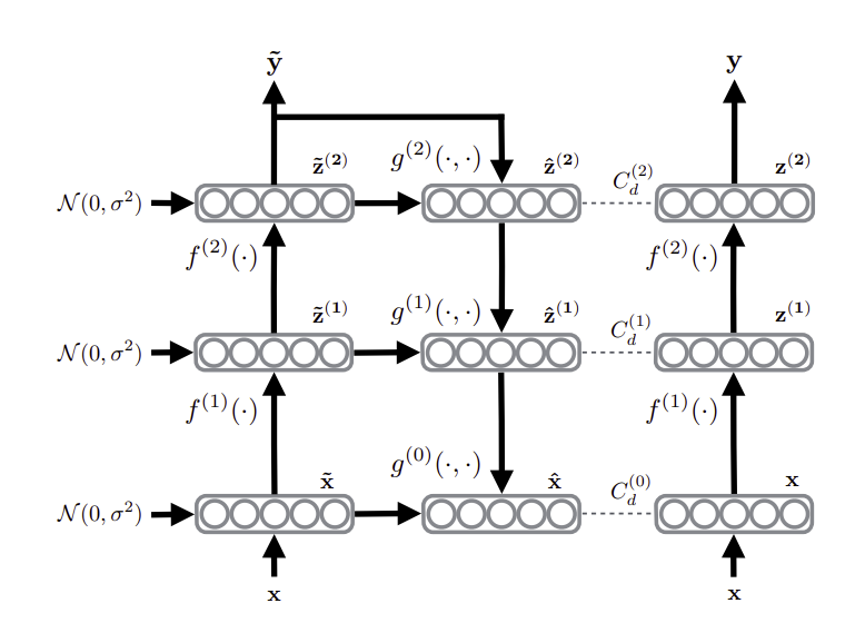
All you really need to understand is that, given an image \(x\), you feed it through an encoder \(f(\cdot)\) with random noise added to the activations \(\tilde{z}^{(i)}\) and get a label \(\tilde{y}\). Repeat the same pipeline with no noise added to get activations \(z^{(i)}\).
Finally, want to train our decoder \(g(\cdot)\) to map \(\tilde{z}^{(i)}\) to \(\hat{z}^{(i)} = g(\tilde{z}^{(i)})\) that minimizes the MSE to the activations from the clean activations \(z^{(i)}\):
\[L= \left|\left|g(\tilde{z}^{(i)}) - z^{(i)}\right|\right|^2_2 =\left|\left|\hat{z}^{(i)} - z^{(i)}\right|\right|^2_2\]Training labels here are completely optional, which is a bit of shortcoming. As the Mean Teacher paper states:
Since the model itself generates targets, they may very well be incorrect. If too much weight is given to the generated targets, the cost of inconsistency outweighs that of misclassification, preventing the learning of new information.
Self-supervision with temporal ensembling
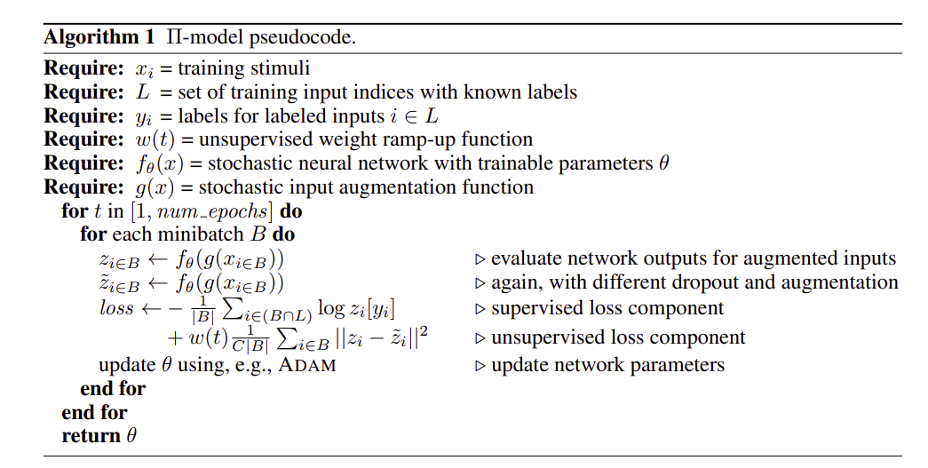
\(\Pi\) networks

The main idea is to add different noise to the input \(x\) with targets \(y\), to get \(x_1\) and \(x_2\), and put this into a network with dropout. Then you simply optimize the cross entropy on one of the samples, and minimize the squared difference between the logits \(z_1 = f(x_1)\) and \(z_2 = f(x_2)\) of both samples:
\[L = \text{cross_entropy}(z_1, y) + w(t)||z_1 - z_2||^2_2\]You may also notice a weighting term \(w(t)\) on the MSE. This term starts off low, to allow the cross entropy term to help the model learn a supervised representation. It linearly increases in order to give more weightage to the SSL terms at later stages of the model training.
\(\Pi\) network + temporal ensembling

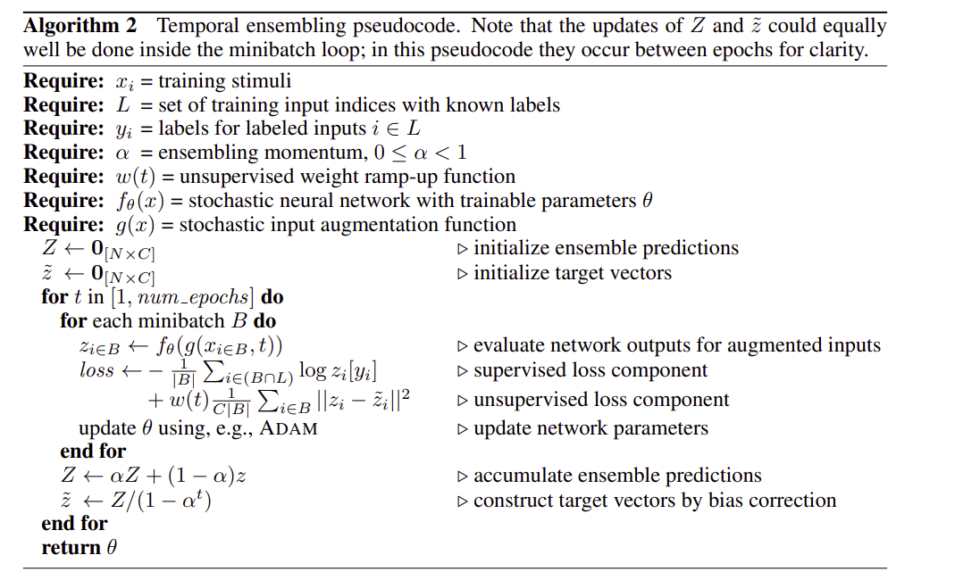
For temporal ensembling, we take our inputs \(x\) (with some data augmentation) and produce logits \(z = f(x)\). We also maintain an EMA of our past predictions on this datapoint \(x\). So say \(x\) as been seen 4 times in the previous 4 epochs with different augmentations (assuming each epoch cycles through the data with no replacement), we’ll have four different sets of logits \([z_1, z_2, z_3, z_4]\). We also have observed the logits \(z_5\), once we saw \(x\) on our current epoch 5.
We then compute an EMA \(\tilde{z}_4\)of these past 4 logits, and we have the loss term
\[L = \text{cross_entropy}(z_5, y) + w(t)||z_5 - \tilde{z}_4||^2_2\]Then, we update our EMA for this datapoint:
\[\tilde{z}_5 = \beta \tilde{z}_4 + (1-\beta)z_5\]Of course, we don’t actually keep a storage of logits \([z_1, z_2, \dots, z_N]\) for each time we see datapoint \(x\), we can just store the EMA and update it in-place.
The main idea here is that, the EMA offers a more robust embedding since it incorporates previous context/models. By ensembling these embeddings via EMA, and supervising on that, we can observe much better performance.

Here’s the full algorithm if you’re interested
Here’s the big issues with this:
- The time it takes for the EMA to actually be rich enough to provide a good representation takes a lot of time. Say it takes 10 logits in the EMA for a datapoint to actually be useful, that means 10 epochs, so this is roughly \(O(10\cdot D)\). This can be a LOT of time if \(D\) is large.
- For modern datasets with many classes, this means you need to keep \(O(C^2)\) floats in memory. Where \(C\) is the number of classes and dimension of the logits.
Mean teachers are better role models
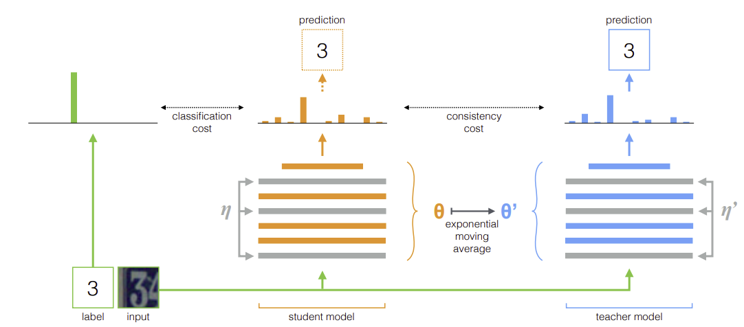
The idea here is simple. Given an input \((x,y)\), student parameters \(\theta_{student}\) and teacher parameters \(\theta_{teacher}\). Compute their respective outputs \(f(x; \eta_{student}, \theta_{student})\), \(f(x; \eta_{teacher}, \theta_{teacher})\), where the \(\eta 's\) are some gaussian noise that we add to the layers of both models.
Then, compute a classification loss on the student logits, and a consistency loss on the teacher and student logits.
\[L = \text{cross_entropy}(f(x; \eta_{student}, y)) + ||f(x; \eta_{student}, \theta_{student}) - f(x; \eta_{teacher}, \theta_{teacher})||_2^2\]Finally, we update the student model with GD and update the EMA of our teacher model:
\[\theta_{student} = \theta_{student} - \alpha \nabla_L(\theta{student})\] \[\theta_{teacher} = \beta \theta_{teacher} + (1-\beta) \theta_{student}\]The main idea here is that we keep a EMA of the student models, and use that as the teacher.
Turns out this empirically did much better than state of the art, especially in the low-label count regime.
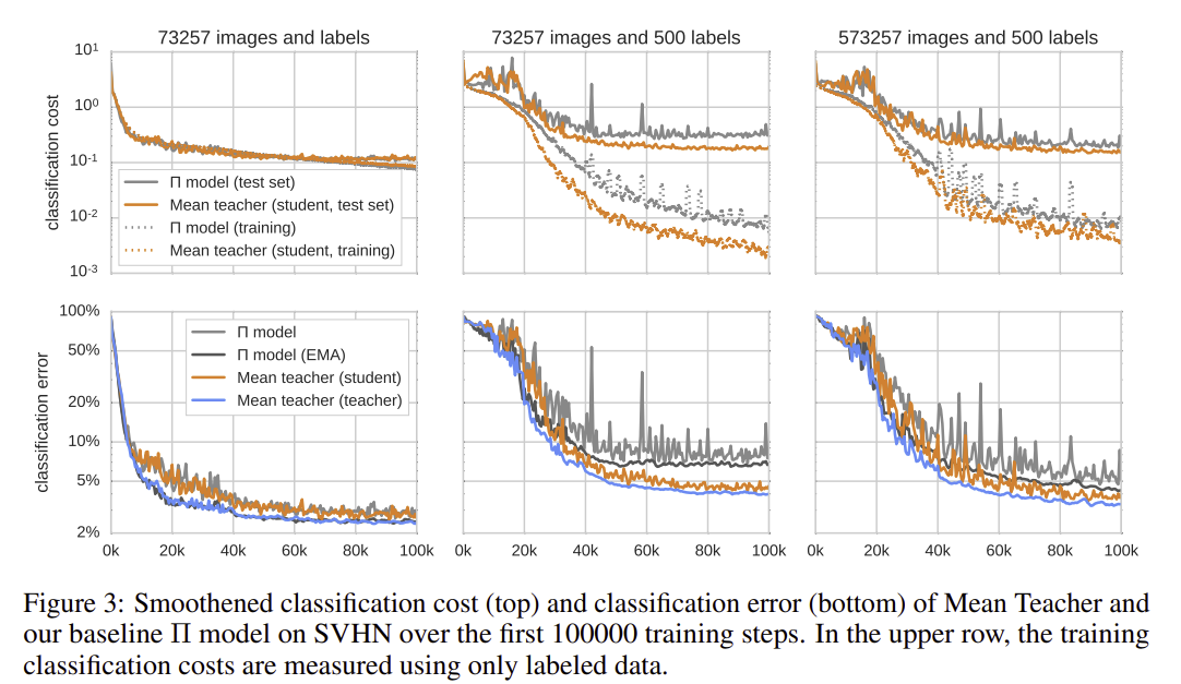
This fixes the main issue that temporal ensembling had with slow updates + data storage, as now the teacher is being updated each weight update, and we don’t need to store a lot of EMAs. The only requirement is that the student fits in VRAM twice.
Wrap up
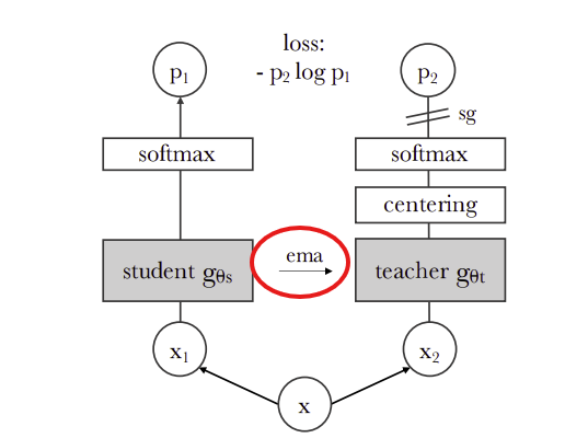
This roughly traces the paper trail for what inspired the EMA + two image augmentation for modern SSL. The goal is to offer continous per-batch supervision using a teacher model, which turns out to work well as an EMA. Additionally different augmentation is to keep the model features robust to image perturbations.
The questions I have after this is:
- In what situations does this break? I guess that this all is very sensitive to \(\beta\), the choice of augmentations, different schedules for hyperparameters etc… I’m wondering what causes this framework to become unstable.
- Mean teacher has explicit supervision on the targets, but modern SSL does not. How did we remove reliance on labels entirely?