Inverse Transform Sampling in NeRF
Problem Setup
I was working on my implementation of NeRF and I read section 5.2 (Hierarchical Sampling). As discussed in the paper we have t-values \((t_1, \dots, t_{N_c})\), and we compute weights \(w_1, \dots, w_{N_c}\) as:
\[w_i=T_i\left(1-\exp \left(-\sigma_i \delta_i\right)\right)\]They then normalize these weights to produce a piecewise constant PDF:
\[\hat{w}_i = \frac{w_i}{\sum_{j=1}^{N_c} w_j}\]The authors propose using inverse transform sampling to sample t-values along the this ray around points that have a high \(\hat{w}_i\).
When I read this my understanding of inverse transform sampling was limited to what’s described here.
However, none of these sampling techniques apply here because we don’t have the analytic form of an inverse CDF \(F^{-1}(x)\).
Therefore, we need to construct this CDF and a method of evaluating it.
A first pass
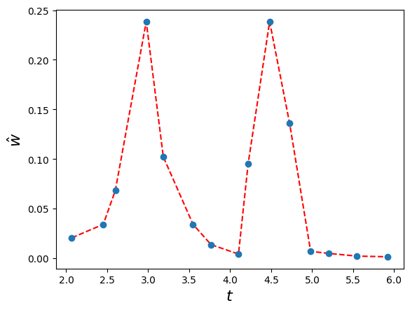
Let’s start simple, lets say we have the following ordered set of (t-value, \(\hat{w}\)) pairs \((t_1, \hat{w}_1), \dots, (t_{N_c}, \hat{w}_{N_c})\), such that \(\sum_{j=1}^{N_c} \hat{w}_j = 1\) and \(t_i < t_{i+1}\).
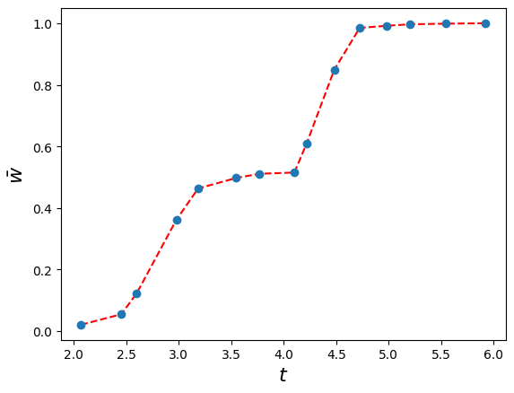
Okay, now let’s compute the cumulative sum. We will now have points \((t_1, \bar{w}_1), \dots, (t_{N_c}, \bar{w}_{N_c})\) where \(\bar{w}_i = \sum_{j=1}^{i} \hat{w}_j\) (note the last point should have a height of 1).
Now, I want to somehow use this to perform inverse transform sampling, that is, mapping \(u \sim U[0,1]\) to a t-value \(t_u\).
My first guess is to find the neighboring points on the cumulative sum function \((t_{left}, \bar{w}_{left}), (t_{right}, \bar{w}_{right})\) such that \(\bar{w}_{left} \leq t \leq \bar{w}_{right}\). With this, we can compute \(t_u\) as:
\[t_u = (t_{right} - t_{left}) \cdot r + t_{left}, \hspace{0.5cm} r= \frac{u - \bar{w}_{left}}{\bar{w}_{right} - \bar{w}_{left}}\]Here are some visualizations of this procedure:
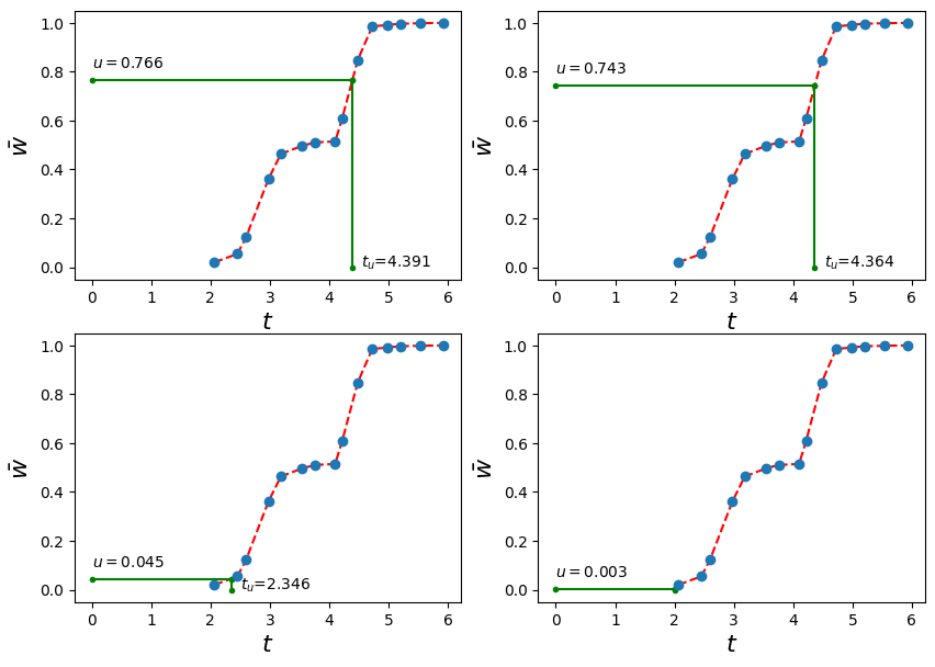
However, notice what happens if \(u < \bar{w}_1\), we cannot find a \(\bar{w}_{left}\) such that \(\bar{w}_{left} \leq u\). Therefore this method doesn’t work when \(u < \bar{w}_1\).
An online solution
I look around on the internet for how people implement this, and I found Krishna Murthy’s NeRF Implementation. The rest of the post will be going over how this is implemented.
Krishna Murthy instead does the following:
- Take your t-values \((t_1, \dots, t_{N_c})\) and compute a new list of \(N_c-1\) points
-
Take weights \((w_2, \dots, w_{N_c - 1})\). Note that they are not normalized. then replace each \(w_i\) with \(\hat{w}_i = \frac{w_i}{\sum_{j=2}^{N_c - 1} w_i}\). This is a list of \(N_c - 2\) probabilities. Append a 0 to the beginning of the list to get \((0, \hat{w}_2, \dots, \hat{w}_{N_c -1})\). Finally like before, replace each \(\hat{w}_i\) with \(\bar{w}_i = \sum_{j=2}^{i} \hat{w}_j\) to get \((0, \bar{w}_2, \dots, \bar{w}_{N_c -1})\). We now have \(N_c - 1\) probabilities.
-
Pair up these \(N_c -1\) points and probabilities to get:
Notice that the first point has a y value of 0, and the last has a y value of \(\bar{w}_{N_c-1} =1\) by definition. We now are able to find a left and right neighbor for all \(u \in [0,1]\), solving our previous problem.
Let’s visualize what this function looks like compared to our previous one.
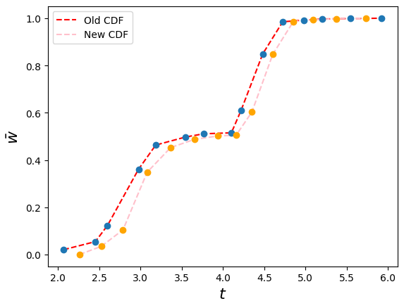
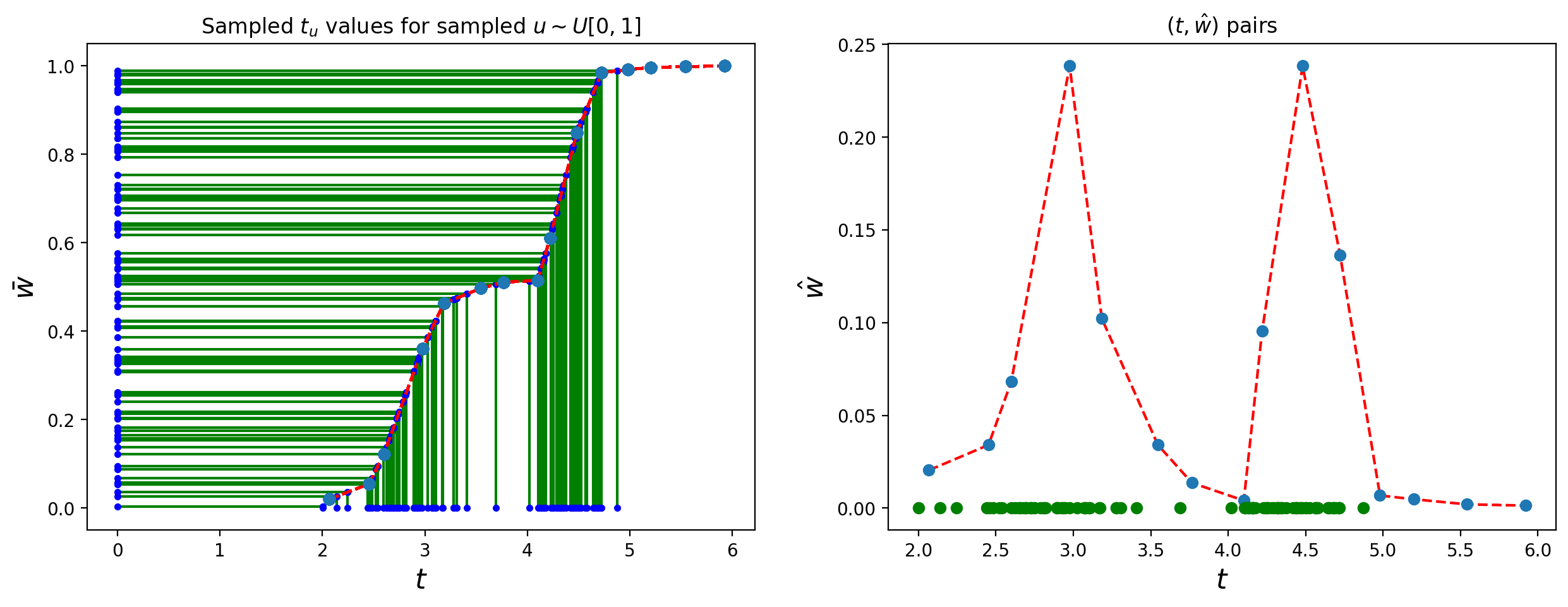
As you can see, it’s very similar to our previous attempt at a CDF and puts a lot of density around the regions with t-values that have a high probability. To illustrate this, I sampled 100 values \((u_1, ..., u_100)\) and computed \(t_{u_i}\) for each of them using the inverse transform sampling scheme I described earlier. On the left of the plot below, Each \(u_i\) is plotted in blue on the y-axis, and the corresponding \(t_{u_i}\)’s are also plotted in blue on the x axis.
On the right of the plot below, I’ve plotted the original t-values and their normalized weights, exactly the same as the first figure in this blogpost. However, I’ve added the green dots on the x-axis which correspond to each of the \(t_{u_i}\)’s. As you can see, most of them lie in high density regions of the ray. This shows that with this method, we’re able to sample t-values from high density regions along the ray using inverse transform sampling.
